2D Channel Flow with a Cylinder#
This example solves the two-dimensional incompressible Navier-Stokes equations in a channel using MOLE mimetic operators and a projection (pressure-correction) method.
The cylinder obstacle is introduced as a masked no-slip region inside the channel. To make things easy, the current implementation uses an axis-aligned masked block of cells rather than a fitted curved boundary. The purpose of this example is to show how MOLE operators can be combined to build a transient incompressible flow solver in a direct and compact way.
Governing Equations#
We solve the incompressible Navier-Stokes equations
where \(\mathbf{u} = (u,v)\) is the velocity field, \(p\) is the pressure, \(\rho\) is the density, and \(\nu\) is the kinematic viscosity.
Spatial Domain#
The computational domain is
The default grid is
\(m = 481\) cells in the \(x\)-direction
\(n = 121\) cells in the \(y\)-direction
The Reynolds number is defined through
with the default values
\(Re = 200\)
\(U_{\mathrm{init}} = 1\)
Initial and Boundary Conditions#
Initial Conditions#
At \(t = 0\),
in the fluid region, and the masked obstacle region is initialized with
Velocity Boundary Conditions#
Inlet (left): Dirichlet inflow
\[ u = U_{\mathrm{init}}, \qquad v = 0 \]Outlet (right): zero streamwise gradient
\[ \frac{\partial u}{\partial x} = 0, \qquad \frac{\partial v}{\partial x} = 0 \]Top and bottom walls: no-slip
\[ u = 0, \qquad v = 0 \]Obstacle mask: no-slip
\[ u = 0, \qquad v = 0 \]
Pressure Boundary Conditions#
During the pressure Poisson step,
Outlet (right): reference pressure
\[ p = 0 \]All other boundaries: homogeneous Neumann
\[ \frac{\partial p}{\partial n} = 0 \]
Numerical Method#
A projection method is used to enforce incompressibility.
This is the same overall time-stepping strategy used in both the MATLAB/Octave and C++ implementations.
Time Integration#
The momentum equation is advanced with a mixed time discretization:
the convective term is treated explicitly with AB2 (Adams-Bashforth 2)
the first time step uses AB1
the diffusive term is treated implicitly with Crank-Nicolson
The convective term is nonlinear, so an explicit AB2 treatment keeps the method simple and avoids solving a nonlinear system at each time step. The diffusive term is linear and is treated with Crank-Nicolson to obtain a stable and second-order accurate semi-implicit update.
As a result, the intermediate velocity solve uses the matrices
which are the Crank-Nicolson diffusion matrices used in the Helmholtz-type solves for \(u^*\) and \(v^*\).
Intermediate Velocity#
An intermediate velocity \(\mathbf{u}^*\) is computed first from the momentum equation using the explicit convective update and the semi-implicit diffusive update.
Pressure Poisson Equation#
The pressure is then obtained from
Velocity Correction#
The velocity is corrected by
Re-application of Velocity Boundary Conditions and Mask#
After the pressure correction step, the code re-applies the velocity boundary values and the obstacle mask.
This is done because the projection step updates the full cell-centered velocity field. Re-applying these values ensures that the final updated velocity satisfies the intended inlet, wall, outlet, corner, and masked-region constraints exactly.
Role of the MOLE Operators#
This example is intended to highlight how MOLE operators are used in an incompressible flow solver.
The main operators are
Laplacian \(L\): used for viscous diffusion
Divergence \(D\): used in the convective flux form and in the pressure Poisson right-hand side
Gradient \(G\): used in the pressure correction step
Interpolation operators: used to map between cell-centered values and face-based quantities for flux evaluation and projection
These operators are combined to build
the Crank-Nicolson diffusion operators
the pressure Poisson operator
the interpolation maps needed for face fluxes and pressure-gradient correction
Running the Example#
After building the C++ examples, run
cd <mole-repo>/examples/cpp
../../build/examples/cpp/cylinder_flow_2D
MATLAB and C++ Versions#
MATLAB/Octave and C++ versions of this example are provided with the same problem setup and the same overall projection-method structure. In particular, both versions use
AB2 for the convective term
AB1 at the first step
Crank-Nicolson for the diffusive term
a pressure Poisson solve followed by velocity correction
This makes it easier to compare the two implementations and to see how the same MOLE operators are used in each language.
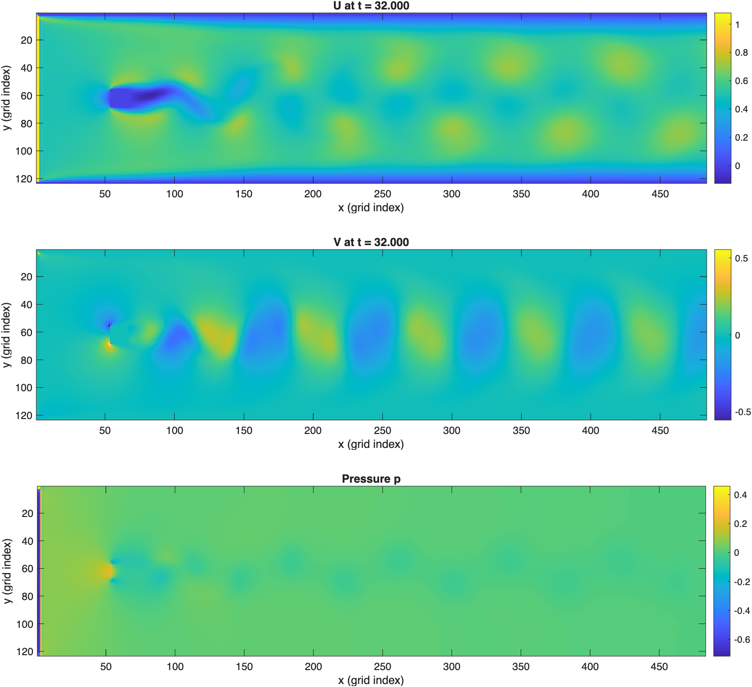
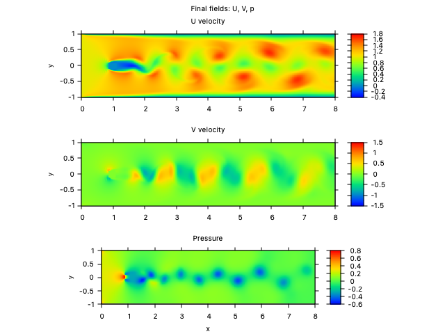
Results#
C++ result#
MATLAB result#